Validation / 4 of 10

Cantilever beam, quadratic hexahedra

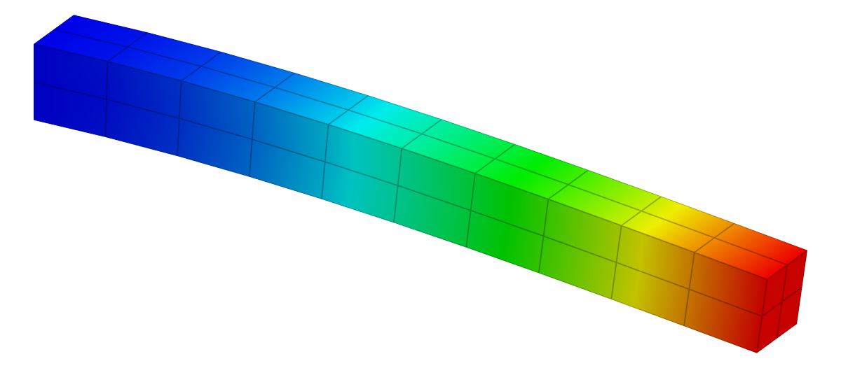
The cantilever again, on a mesh four times coarser in each direction (10 × 2 × 2), with quadratic elements instead of linear ones. The case checks KoFEM's second-order element path and shows why element order matters in bending.

Tip deflection δ; reference δ = P·L³ / (3·E·I)
Reference	KoFEM	Difference
−1.9048 mm	−1.9398 mm	+1.84 % within ±4 %

Open in KoFEMOpens the solved model in the app.

The problem

Beam of span L along x, b × h section, I = b·h³/12. Sketch, not to scale; thin lines show the element mesh.

$L$	1000 mm
$b \times h$	100 × 100 mm
$E$	210 GPa
$ν$	0.3
$P$	10 kN

Supports	x = 0 face fixed (Ux, Uy, Uz).
Load	P in −y as a force on the x = L face.
Measured	Mean y-displacement of the x = L face vertices.

Analytical solution

Euler–Bernoulli beam theory assumes that cross-sections stay plane and perpendicular to the deformed axis, which neglects shear deformation. Take $w (x)$ as the deflection, positive upwards, with the load $P$ acting downwards at the tip. Equilibrium of the part beyond a section $x$ gives the bending moment

M (x) = - P (L - x),

and the curvature is proportional to it:

E I \frac{d^{2} w}{d x^{2}} = M (x), I = \frac{b h^{3}}{12} .

Integrating twice with the clamp conditions $w (0) = 0$ and $\frac{d w}{d x} (0) = 0$ gives the deflection curve

w (x) = - \frac{P x^{2}}{6 E I} (3 L - x),

and at the tip

δ = w (L) = - \frac{P L^{3}}{3 E I} .

For this beam $I = 8.3333 \times 10^{6} {mm}^{4}$ and $δ = - 1.9048 mm$ .

Timoshenko beam theory adds the shear deformation that Euler–Bernoulli leaves out. For a cantilever with a tip load it adds a second term,

δ_{s} = - \frac{P L}{κ G A}, κ = \frac{5}{6}, G = \frac{E}{2 (1 + ν)},

which is 0.78 % of the bending term for this beam (span ten times the depth). A converged 3-D solid model should therefore deflect slightly more than $P L^{3} / (3 E I)$ .

Finite element model

Mesh	10 × 2 × 2 grid: 40 quadratic 27-node hexahedra (P2)
Unknowns	525 nodes, 1,575 degrees of freedom
Material	Linear elastic, isotropic
Solver	KoFEM engine (MFEM), the WebAssembly build the app runs: engine-5ceb743373dd

A quadratic hexahedron has 27 nodes: at its corners, edge midpoints, face centres and centre. The displacement varies quadratically along each edge, so an element can curve. Clamping the $x = 0$ face fixes all of its nodes, including the mid-edge and mid-face ones. The 40 elements have 525 nodes and 1,575 unknowns, about half the 3,075 of the linear mesh. The tip load is a force on the end face, integrated with the quadratic shape functions, so the mid-side nodes carry their share.

Results

Quantity	tip deflection δ
Reference	δ = P·L³ / (3·E·I) = −1.9048 mm (Euler–Bernoulli beam theory)
KoFEM	−1.9398 mm
Difference	+1.84 % within ±4 %

Mesh convergence: Cantilever beam, P1 vs. P2

P1 (linear)P2 (quadratic)below the referenceabove

Difference from the reference on refined meshes, logarithmic axes. The ringed point is this example's mesh.

Linear elements lock in bending and approach from far below; quadratic ones are within a few percent on every mesh and level off slightly above the reference, since Euler–Bernoulli theory neglects shear deformation.

Data

Order	Mesh	DOFs	KoFEM	Difference
P1 (linear)	10 × 1 × 1	132	−1.2339 mm	−35.22 %
P1 (linear)	20 × 2 × 2	567	−1.6682 mm	−12.42 %
P1 (linear)	40 × 4 × 4 (this example)	3,075	−1.8378 mm	−3.51 %
P1 (linear)	80 × 8 × 8	19,683	−1.8879 mm	−0.88 %
P2 (quadratic)	5 × 1 × 1	297	−1.8847 mm	−1.05 %
P2 (quadratic)	10 × 2 × 2 (this example)	1,575	−1.9398 mm	+1.84 %
P2 (quadratic)	20 × 4 × 4	9,963	−1.9330 mm	+1.48 %

Discussion

On this coarse mesh the deflection differs from the Euler–Bernoulli value by +1.84 % and is close to the Timoshenko value that includes shear deformation, $- 1.9196 mm$ . A quadratic element can represent a linearly varying bending strain exactly: its edges curve, so it bends without parasitic shear and does not lock.

Linear elements on meshes this coarse lock badly. In the convergence study above, the error is −35.22 % with 10 × 1 × 1 linear elements and −12.42 % with 20 × 2 × 2; the quadratic series is within a few percent on every mesh. For bending-dominated parts, quadratic elements give more accuracy per unknown.

Reproduce

In the app: open the model, then Studies → Static 1 → Run static solve, select the result plot and set Field to Uy. The Result summary shows Min Uy -1.940e+0 mm.

From a clone (Node.js 20+, bash, curl), this solves the model with the same engine and prints its line:

git clone https://github.com/mkofler96/KoFEM.git && cd KoFEM
bash scripts/fetch-wasm-engine.sh
node examples/validation/run.mjs --case cantilever-p2

Case                                  Quantity                                  FE   Reference     Err%  Tol%  Status
Cantilever beam, quadratic hexahedra  tip deflection δ                     -1.9398     -1.9048    +1.84     4  PASS

References

J. M. Gere and B. J. Goodno, Mechanics of Materials, Cengage Learning: axially loaded members, torsion, deflections of beams.
S. P. Timoshenko, “On the correction for shear of the differential equation for transverse vibrations of prismatic bars”, Philosophical Magazine 41 (1921) 744–746.
R. D. Cook, D. S. Malkus, M. E. Plesha and R. J. Witt, Concepts and Applications of Finite Element Analysis, 4th ed., Wiley, 2002.
T. J. R. Hughes, The Finite Element Method: Linear Static and Dynamic Finite Element Analysis, Dover, 2000.

KoFEM is research software and is not certified for safety-critical design. It solves linear-static, linear-elastic problems. Check results that matter against your own references.